PITCH DETECTION
kevin_thibedeau writes
There is a good way to make the
harmonic product spectrum more robust to the effects of noise. You
generate a synthetic spectrum starting from a histogram of zero crossing
intervals that has been "smeared" back into a continuous signal with
Gaussian peaks by applying a kernel density estimate. The result can
then be passed through the HPS to find the fundamental. The decorrelated
zero crossings caused by noise are much less problematic than working
with the HPS of the original signal.
Also, an overview here: http://obogason.com/fundamental-frequency-estimation-and-machine-learning/
Original link:https://news.ycombinator.com/item?id=10757879
PEAK DETECTION
John on comp.dsp writes (https://groups.google.com/forum/#!topic/comp.dsp/MqSJjoaq8Hg)
It is entirely inappropriate for some problems, but one peak-picker that I use sometimes is a three segment sliding window:
LLLLLLLLLLCCCCCRRRRRRRRRR
When the maximum of window C is in the middle of C, and that maximum
exceeds max(f(L),f(R)), then a peak at the middle of C is declared. The
function f can be mean(L) or max(L) or something else. The window
lengths are tuned to your requirements
Lito on comp.dsp writes
For a series with well behaved peaks the following
has worked for me. What it lacks in efficiency it
it makes up for with reliability.
function peaks(x,region,thresh)
value,index = max(x)
while value > thresh
add value, index to list
zero out region about index
value,index = max(x)
endwhile
return list
Monday, December 9, 2013
Monday, October 28, 2013
Git snippets
REMOVE LARGE FILES (all .pkl files in this case)
git filter-branch --index-filter 'git rm --cached --ignore-unmatch *.pkl' --tag-name-filter cat -- --all
ARTICLE ON GIT SUBMODULES
http://chrisjean.com/2009/04/20/git-submodules-adding-using-removing-and-updating/
Basically, git submodule add https://kastnerkyle@github.com/kastnerkyle/RNNLIB RNNLIB
git filter-branch --index-filter 'git rm --cached --ignore-unmatch *.pkl' --tag-name-filter cat -- --all
ARTICLE ON GIT SUBMODULES
http://chrisjean.com/2009/04/20/git-submodules-adding-using-removing-and-updating/
Basically, git submodule add https://kastnerkyle@github.com/kastnerkyle/RNNLIB RNNLIB
Saturday, September 21, 2013
Adjusting Low Volume in Linux
QUIET RIOT
First, try running
alsamixer
from the command line. If there is still some headroom on any of the sliders, bump them to 100%. Sometimes there are weird interactions between the different volume sliders, and making them all 100% could increase you output volume.
IT AIN'T ENOUGH
For even more volume, we can head to the commandline.
pacmd list-sinks
will list all possible sinks for volume increases on your system. To bump my volume to approximately 200% (100% is 65536), I used:
pacmd set-sink-volume alsa_output.pci-0000_00_1b.0.analog-stereo 125000
This will increase noise to some extent (looking into some good ways to filter it), but at least those quiet sounds can now be heard!
http://askubuntu.com/questions/219739/adjust-max-possible-volume-in-pulseaudio
Wednesday, July 17, 2013
Python code snippets
EXCELLENT COVERAGE OF MATPLOTLIB
http://nbviewer.ipython.org/urls/raw.github.com/jrjohansson/scientific-python-lectures/master/Lecture-4-Matplotlib.ipynb
ZIP A LIST INTO SUBGROUPS
izip(*[iter(l)]*size)
zip(*[imap(func)]*size)
BETTER EXAMPLE CONTROLLING SSH WITH PEXPECT AND PXSSH
#!/usr/bin/env python
import pxssh
def getLine(password="password", hostname="host"):
try:
s = pxssh.pxssh()
username = "root"
s.login (hostname, username, password)
s.sendline ("echo 'Hello World'") # run a command
s.prompt() # match the prompt
line = s.before
s.logout()
return line
except pxssh.ExceptionPxssh, e:
print "pxssh failed on login."
print str(e)
print getLine()
EXAMPLE OF CONTROLLING SSH IN PURE PYTHON WITH CORE LIBS
#!/usr/bin/env python
import pty
import os
import sys
import time
pid,fd = pty.fork()
if pid==0:
os.execv("/usr/bin/ssh",["/usr/bin/ssh","root@host","echo 'Hello World!' | awk '{print $2}'"])
else:
password = 'password\n'
print "Child says",os.read(fd,1024).strip()
print "Child took",os.write(fd,password)
time.sleep(1)
print "Child says",os.read(fd,1024).strip()
#SSH uses pty instead of stdin to communicate
#http://www.gossamer-threads.com/lists/python/python/56425
Thursday, May 30, 2013
Statistics Tidbits
Bayes Rule Refresher
Choosing a statistical test
http://imgur.com/Ctug4Dr
Aikake Information Criterion
Maximum Likelihood
$AIC = -2*logL(\theta|y) + 2k$
$k = $ total number of parameters
Least Squares
$AIC = n*log(\frac{RSS}{n}) + 2k$
$RSS = SSE = \sum(y - h(x))^2$
$ n = $ number of samples
http://www4.ncsu.edu/~shu3/Presentation/AIC.pdf
http://en.wikipedia.org/wiki/Residual_sum_of_squares
Matrix Form Pointwise Distances
$d_ij = ||x_i - y_j||^2 = ||x_i||^2 + ||y_j||^2 - 2<X_i,y_j>$
means that
$D = X + Y - 2X'Y$
Take the norm of X and Y i.e. X*X' or dot(X,X')
Normalize and calculate covariance
A * A.T (Hermitian!) / sqrt(diag(A.T * A) * diag(A.T * A).T)
http://statinfer.wordpress.com/2011/11/14/efficient-matlab-i-pairwise-distances/
Rolling stats
http://stackoverflow.com/questions/1058813/on-line-iterator-algorithms-for-estimating-statistical-median-mode-skewnes
Current Links for Stats in Python
http://r.789695.n4.nabble.com/Ornstein-Uhlenbeck-td2991060.html
http://camdavidsonpilon.github.io/Probabilistic-Programming-and-Bayesian-Methods-for-Hackers/
http://blog.yhathq.com/posts/estimating-user-lifetimes-with-pymc.html
http://robjhyndman.com/hyndsight/crossvalidation/
Here's another useful way to state the Bayes' rule for conditional probability (it just expands on what the OP wrote):

Note that here (1) is just the definition, (2) is a simple application of Bayes rule that we already know, and (3), (4) are various ways to rewrite (1) using factorization rules of the type P(ABC) = P(A|BC)P(B|C)P(C). Mentally, I find the following procedure useful:
This makes sense intuitively, if you think of conditioning as procedure of renormalizing the sample space in various ways. It's reasonable that you should be able to use Bayes' rule in the same way whether or not the probability space has been renormalized by conditioning.
|
Choosing a statistical test
http://imgur.com/Ctug4Dr
Aikake Information Criterion
Maximum Likelihood
$AIC = -2*logL(\theta|y) + 2k$
$k = $ total number of parameters
Least Squares
$AIC = n*log(\frac{RSS}{n}) + 2k$
$RSS = SSE = \sum(y - h(x))^2$
$ n = $ number of samples
http://www4.ncsu.edu/~shu3/Presentation/AIC.pdf
http://en.wikipedia.org/wiki/Residual_sum_of_squares
Matrix Form Pointwise Distances
$d_ij = ||x_i - y_j||^2 = ||x_i||^2 + ||y_j||^2 - 2<X_i,y_j>$
means that
$D = X + Y - 2X'Y$
Take the norm of X and Y i.e. X*X' or dot(X,X')
Normalize and calculate covariance
A * A.T (Hermitian!) / sqrt(diag(A.T * A) * diag(A.T * A).T)
http://statinfer.wordpress.com/2011/11/14/efficient-matlab-i-pairwise-distances/
Rolling stats
http://stackoverflow.com/questions/1058813/on-line-iterator-algorithms-for-estimating-statistical-median-mode-skewnes
Current Links for Stats in Python
http://r.789695.n4.nabble.com/Ornstein-Uhlenbeck-td2991060.html
http://camdavidsonpilon.github.io/Probabilistic-Programming-and-Bayesian-Methods-for-Hackers/
http://blog.yhathq.com/posts/estimating-user-lifetimes-with-pymc.html
http://robjhyndman.com/hyndsight/crossvalidation/
https://www.leinenbock.com/tag/statsmodels/
http://nbviewer.ipython.org/urls/raw.github.com/carljv/Will_it_Python/master/MLFH/ch8/ch8.ipynb
http://nbviewer.ipython.org/urls/github.com/weecology/progbio/raw/master/ipynbs/statistics.ipynb
http://wiki.answers.com/Q/What_does_a_high_t_statistic_mean
http://stackoverflow.com/questions/13452353/multiple-correlation-in-python
http://stats.stackexchange.com/questions/4422/small-sample-linear-regression-where-to-start
Tuesday, April 2, 2013
Installing the Redhawk SDR framework
WHAT IS IT?
Redhawk SDR is a new SDR framework, in the vein of GNU Radio Companion and the OSSIE framework, for quickly developing and deploying signal processing algorithms. This U.S. Gov't backed software has extensive support for creating radio flows for a single computer or distributing your SDR processing chain across networked hardware, and has been used in many commercial applications. It will also be incorporating the existing work done under the banner of GNU Radio Companion and OSSIE. See more at www.redhawksdr.org
FLY ON YOUR WINGS (LIKE AN EAGLE)
The first step (or at least the easiest way to get going) is to install CentOS 6.{1-3} x86_64. Redhawk comes in rpm packages, so I am sure other flavors of RedHat Linux could work, but I personally used CentOS 6.3 x86_64 for this tutorial. Of course, some of the difficulties I experienced may be alleviated by a better repository package set like Fedora has.
To install the redhawk software, take the code from the GitHub link below and paste into a bash script, then set executable permissions with chmod +x <scriptname>. I have the latest copy of this posted on my GitHub for Redhawk utilities.
Once this script completes, you should see a folder called redhawkIDE in your home directory. Enter this folder, then type ./eclipse. This should launch the Redhawk IDE, which allows you to create components and blocks to do SDR task.
ODD FUTURE
I am planning to include support for 32bit and 5.x installs of CentOS in the get_redhawk.sh script at some point, but for now only CentOS 6.x 64bit is supported.
Redhawk has begun to integrate GNU Radio components into the framework, which will hopefully bring rtl-sdr support. This should support the E4000 and R820T digitizers, so that we can quickly begin to use the Redhawk SDR environment for some real projects. For now, the only way I can see to get rtl-sdr working with Redhawk is through a nasty hack - make a FIFO and write data from rtl-sdr to that... I will be posting on this in the near future.
Tuesday, March 12, 2013
Introduction to Machine Learning, Part 2: Linear Regression
NUMERO DOS
Continuing our exploration of machine learning, we will discuss the use of basis functions for regression analysis. When presented with an unknown dataset, it is very common to attempt to find trends or patterns. The most basic form of this is visual inspection - how is the data trending? Does it repeat in cycles? Can we predict future data given some past events? The mathematical approach to this "trend finding" is called regression, or line fitting. As we will see, it is possible to fit more than a simple straight line, and the general technique of regression is very effective at breaking down many types of data.
DRY DRY DERIVATION
What are some sample functions we might want to perform regression on? Take as an example:
With $x = 1\ldots100$ and no noise, the output $y$ looks like this:


Looking at the function $x^2 - 4x +1$, rearranged as $1-4x+x^2$, we see that this is really a specialization of the general $2$nd order polynomial $w_0 + w_1x + w_2x^2$, with weight vector ${\bf w} = [1, -4, 1]$. If we also abstract the function vector ${\bf x} = \sum\limits_{n=0}^2x^n = [0, x, x^2]$, the result is a function $y({\bf w}, {\bf x}) = w_0 + w_1x_1 + w_2x_2$.
If we think of any $n$th order polynomial, $y({\bf w}, {\bf x})$, it can always be represented by the form.
#!/usr/bin/python
import numpy as np
import matplotlib.pyplot as plot
import math
def gen_dft(m, n, N):
return np.exp(1j*-2*m*n/N)
def gen_polynomial(x, m):
return x**m
N = 10
N_basis = 3
noise_var = B = 5
basis = np.matrix(np.zeros((N,N)), dtype=np.complex64)
xs = np.matrix(range(N)).T
ys = np.square(xs) - 4*xs + 1
wm = ys + np.sqrt(B)*np.random.randn(N,1)
for m in range(N_basis):
for n in range(N):
if m == 0:
basis[m,n] = 1.0
else:
basis[m,n] = gen_polynomial(xs[n], m)
#To use the gen_dft basis, make sure to set N_basis = N
#basis[m,n] = gen_dft(m, n, N)
test_data = t = basis*wm
#Calculate using the Moore-Penrose pseudoinverse using the following formula
#maximum_likelihood = wml = np.linalg.inv(basis.T*basis)*basis.T*t
#Direct calculation appears to have numerical instability issues...
#Luckily the pinv method calculates Moore-Penrose pseudo inverse using SVD
#which largely avoids the numerical issues
maximum_likelihood = wml = np.linalg.pinv(basis)*t
plot.figure()
plot.title("Regression fit using polynomial basis function, number of basis functions = $\$$" + `N_basis` + "$\$$")
plot.plot(ys, 'b')
plot.plot(wm, 'ro')
plot.plot(np.real(wml), 'g')
plot.show()


 There are ways to reduce overfitting by regularizing this operation, using something called the "lasso method". There are also methods for sequential estimation, which avoid large matrix operations for higher order basis matrices. We will instead look at a Bayesian approach to regression, which naturally has regularization properties, and also eliminates most of the large matrix math by making this regression a sequential operation. This will greatly help higher order regression, and falls in line with our earlier approaches from part 1.
Continuing our exploration of machine learning, we will discuss the use of basis functions for regression analysis. When presented with an unknown dataset, it is very common to attempt to find trends or patterns. The most basic form of this is visual inspection - how is the data trending? Does it repeat in cycles? Can we predict future data given some past events? The mathematical approach to this "trend finding" is called regression, or line fitting. As we will see, it is possible to fit more than a simple straight line, and the general technique of regression is very effective at breaking down many types of data.
DRY DRY DERIVATION
What are some sample functions we might want to perform regression on? Take as an example:
$y = x^2 - 4x + 1$

What happens if we look at the same values, distorted by some noise?

Since we know the original function for the data, it is easy to "see" the underlying $x^2 - 4x +1$ (the blue line) is still there, but how can we do this mathematically, and without knowledge of the original generating function?
If we think of any $n$th order polynomial, $y({\bf w}, {\bf x})$, it can always be represented by the form.
$y({\bf w}, {\bf x}) = w_0 + w_1x_1 + w_2x_2+\ldots + w_nx_n$
This can also be represented in matrix form.
$[w_0\ldots w_{n}]\left[ \begin{array}{xmat} 1 & 0 & \cdots & 0\\ 0 & x_1 & \cdots & 0 \\ \vdots & \vdots & \ddots & \vdots \\ 0 & 0 & \cdots & x_n \end{array} \right]$
BASE CAMP 1KM
In fact, going one step further, we see that the vector ${\bf x}$ could really be better generalized as a basis vector - that is, our current vector ${\bf x} = [0, x, x^2] = x^n$ could be generalized with something besides $x^n$. We could use sine waves (Fourier basis), Gaussians, sigmoids, wavelets, or any number of other functions to perform this same regression - in fact, this is the root of the concept of transforms in DSP lingo.
When we talk about linear regression, we are really talking about a linear regression in the basis domain - a linear combination of basis functions multiplied by weighting values, which can be used to approximate the original signal. Since we have learned that we can use nearly any function as a basis, let's change notation from ${\bf x}$ to ${\bf \phi}$, where ${\bf \phi}$ is a function of $x$.
$[w_o\ldots w_{n}]\left[ \begin{array}{phimat} \phi_0(x_1) & \phi_0(x_2) & \cdots
& \phi_0(x_n) \\ \phi_1(x_1) & \phi_1(x_2) & \cdots & \phi_1(x_n) \\ \vdots & \vdots
& \ddots & \vdots \\ \phi_m(x_1) & \phi_m(x_2) & \cdots & \phi_m(x_n)
\end{array} \right]$
The full derivation of the maximum likelihood estimate (MLE) can be found here, but the short and sweet version is that the maximum likelihood estimate of ${\bf w}$ is $(\Phi^T\Phi)^{-1}\Phi {\bf t}$, where $\Phi$ is the general basis matrix defined above, and ${\bf t}$ is a set of test datapoints. These test datapoints are generated by $\Phi {\bf w_m}$, where ${\bf w_m}$ are the measured values (red dots shown in the above figures).
$(\Phi^T\Phi)^{-1}\Phi$ is known as the Moore-Penrose pseudoinverse, and it can be replaced by the matrix inverse $\Phi^{-1}$ if the basis matrix is square (3x3, 100x100, etc.). Let's look at the code.
$(\Phi^T\Phi)^{-1}\Phi$ is known as the Moore-Penrose pseudoinverse, and it can be replaced by the matrix inverse $\Phi^{-1}$ if the basis matrix is square (3x3, 100x100, etc.). Let's look at the code.
#!/usr/bin/python
import numpy as np
import matplotlib.pyplot as plot
import math
def gen_dft(m, n, N):
return np.exp(1j*-2*m*n/N)
def gen_polynomial(x, m):
return x**m
N = 10
N_basis = 3
noise_var = B = 5
basis = np.matrix(np.zeros((N,N)), dtype=np.complex64)
xs = np.matrix(range(N)).T
ys = np.square(xs) - 4*xs + 1
wm = ys + np.sqrt(B)*np.random.randn(N,1)
for m in range(N_basis):
for n in range(N):
if m == 0:
basis[m,n] = 1.0
else:
basis[m,n] = gen_polynomial(xs[n], m)
#To use the gen_dft basis, make sure to set N_basis = N
#basis[m,n] = gen_dft(m, n, N)
test_data = t = basis*wm
#Calculate using the Moore-Penrose pseudoinverse using the following formula
#maximum_likelihood = wml = np.linalg.inv(basis.T*basis)*basis.T*t
#Direct calculation appears to have numerical instability issues...
#Luckily the pinv method calculates Moore-Penrose pseudo inverse using SVD
#which largely avoids the numerical issues
maximum_likelihood = wml = np.linalg.pinv(basis)*t
plot.figure()
plot.title("Regression fit using polynomial basis function, number of basis functions = $\$$" + `N_basis` + "$\$$")
plot.plot(ys, 'b')
plot.plot(wm, 'ro')
plot.plot(np.real(wml), 'g')
plot.show()
As we can see, the approximation with 3 basis functions (2nd order polynomial fit) does a pretty good job of approximating the original function. Let's see what happens if we increase the number of basis functions.


We can see that this fit gets closer to the measured data (red dots), but is actually further from the true signal without noise! This is called overfitting, because our estimate is beginning to fit our measurement, which has noise, rather than the underlying function (the blue line). Let's try another example, using the Fourier basis matrix.
The Fourier basis does a decent job of fitting the line, but still has more error than the polynomial fit with the right number of basis functions. Because the original function is polynomial, we should expect a polynomial basis to give superior results. We are overfitting our polynomial regression by including too many basis functions - in general, we want to fit the smallest number of basis functions while still minimizing overall error.

BAYES ASPIRIN
So how do we actually perform a Bayesian regression? There are some complicated derivations once again (pg 17 and onward here), but the idea is that we make iterative estimates, starting with some prior estimate and a likelihood to get a posterior estimate, which we will use as the prior for the next iteration. Remember, Bayesian is all about $posterior\: =\: likelihood\: \times\: prior$. After iterating through all the data points, we expect our estimate to approach the true generating function, without noise. Let's look at the code.
#!/usr/bin/python
import numpy as np
import matplotlib.pyplot as plot
N = 10
noise_var = B = .2**2
lower_bound = lb = 0.
upper_bound = ub = 5.
xs = np.matrix((ub-lb)*np.random.rand(N)+lb).T
xaxis = np.matrix(np.linspace(lb,ub,num=N)).T
w = np.array([1, -4, 1])
ys = w[0] + w[1]*xaxis + w[2]*np.square(xaxis)
t = w[0] + w[1]*xs + +w[2]*np.square(xs) + np.sqrt(B)*np.random.randn(N,1);
def gen_polynomial(x, p):
return x**p
N_basis = 7
alpha = a = 1.
beta = b = 1./B;
prior_m = np.zeros((N_basis, 1))
m = np.zeros((N_basis, N))
prior_s = np.matrix(np.diag(np.array([a]*N_basis)))
s = np.zeros((N_basis, N_basis))
plot.figure()
for n in range(N):
poly = np.vectorize(gen_polynomial)
basis = poly(xs[n], np.matrix(np.arange(N_basis)))
s_inv = prior_s.I*np.eye(N_basis)+b*(basis.T*basis)
s = s_inv.I*np.eye(N_basis)
#Need to use .squeeze() so broadcasting works correctly
m[:,n] = (s*(prior_s.I*prior_m+(b*basis.T*t[n]))).squeeze()
y = m[0,n] + m[1,n]*xaxis + m[2,n]*np.square(xaxis)
plot.plot(xaxis, y, "g")
prior_m[:,0] = m[:,n].squeeze()
prior_s = s
plot.title("Bayesian regression using polynomial basis function, number of basis functions = $\$$" + `N_basis` + "$\$$")
plot.plot(xaxis, ys, "b")
plot.plot(xs, t, "ro")
plot.plot(xaxis, y, "k")
plot.show()
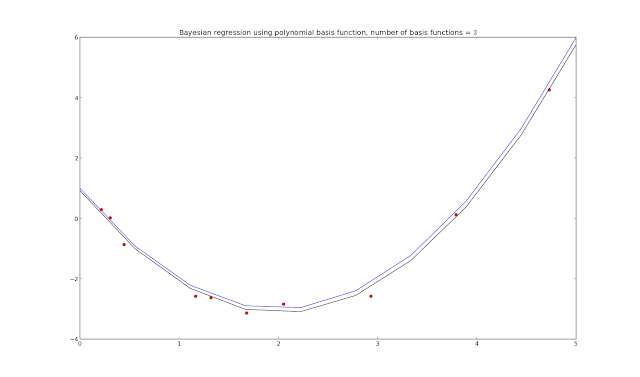 Adding in the progression plots (plot.plot(xaxis, y, "g"))
 The green lines show how the Bayesian regression updates on each iteration through the loop - though unlabeled, we assume that the closer the green line is to the final estimate (black line), the later it ran in the code, with the n = 10 iteration resulting in the final black line shown.
The top part of the code sets up the generating function, also generates samples corrupted by noise. We could set xs differently to get linearly spaced samples (using np.arange(lb,ub,N)) instead of random spacing, but random samples are what Bishop is using in his book and diagrams (Pattern Recognition and Machine Learning, C. Bishop). I also chose to vectorize the basis matrix generation this time - which doesn't actually increase the code speed (in numpy at least), but does turn a multi-line for loop into one line of code.
In fact, looking at page 153 in Bishop's book will give all the formulas used in the processing loop, mapped as follows.

#!/usr/bin/python
import numpy as np
import matplotlib.pyplot as plot
N = 10
noise_var = B = .2**2
lower_bound = lb = 0.
upper_bound = ub = 5.
xs = np.matrix((ub-lb)*np.random.rand(N)+lb).T
xaxis = np.matrix(np.linspace(lb,ub,num=N)).T
w = np.array([1, -4, 1])
ys = w[0] + w[1]*xaxis + w[2]*np.square(xaxis)
t = w[0] + w[1]*xs + +w[2]*np.square(xs) + np.sqrt(B)*np.random.randn(N,1);
def gen_polynomial(x, p):
return x**p
N_basis = 7
alpha = a = 1.
beta = b = 1./B;
prior_m = np.zeros((N_basis, 1))
m = np.zeros((N_basis, N))
prior_s = np.matrix(np.diag(np.array([a]*N_basis)))
s = np.zeros((N_basis, N_basis))
plot.figure()
for n in range(N):
poly = np.vectorize(gen_polynomial)
basis = poly(xs[n], np.matrix(np.arange(N_basis)))
s_inv = prior_s.I*np.eye(N_basis)+b*(basis.T*basis)
s = s_inv.I*np.eye(N_basis)
#Need to use .squeeze() so broadcasting works correctly
m[:,n] = (s*(prior_s.I*prior_m+(b*basis.T*t[n]))).squeeze()
y = m[0,n] + m[1,n]*xaxis + m[2,n]*np.square(xaxis)
plot.plot(xaxis, y, "g")
prior_m[:,0] = m[:,n].squeeze()
prior_s = s
plot.title("Bayesian regression using polynomial basis function, number of basis functions = $\$$" + `N_basis` + "$\$$")
plot.plot(xaxis, ys, "b")
plot.plot(xs, t, "ro")
plot.plot(xaxis, y, "k")
plot.show()


The top part of the code sets up the generating function, also generates samples corrupted by noise. We could set xs differently to get linearly spaced samples (using np.arange(lb,ub,N)) instead of random spacing, but random samples are what Bishop is using in his book and diagrams (Pattern Recognition and Machine Learning, C. Bishop). I also chose to vectorize the basis matrix generation this time - which doesn't actually increase the code speed (in numpy at least), but does turn a multi-line for loop into one line of code.
In fact, looking at page 153 in Bishop's book will give all the formulas used in the processing loop, mapped as follows.
s_inv = ${\bf S}_N^{-1}$
s = ${\bf S}_N$
m[:,n] = ${\bf m}_N$
prior_s = ${\bf S}_0^{-1}$
prior_m = ${\bf m}_0$
Updating the priors with the results of the loop each time, we end up with a reasonable approximation of the generating function as long as N_basis is the same as the generating function. What happens if we don't use the right value for N_basis?

Bad things, it turns out. Instead of an overfitting problem, we now have a model selection problem - if we don't choose N_basis right, we won't converge to the right answer!
AUTO MODELING AND DETAILING
We really want to automate this model selection process, as scientists are too busy traveling the world and winning awards to babysit their award-winning scientific models. Luckily, there is a formula for calculating Bayesian model evidence - the model that maximizes this function should be the best choice! See the notes here (PDF) for more details, starting with slide 41.
${\large {\bf A} = {\bf S}_N^{-1} = \alpha {\bf I} + \beta {\bf \Phi}^T{\bf \Phi}}$
${\large {\bf m}_N = \beta{\bf A}^{-1}{\bf \Phi}^T{\bf t}}$
${\large E({\bf m}_N) = \frac{\beta}{2}||{\bf t}-{\bf \Phi}{\bf m}_N||^2+\frac{\alpha}{2}{\bf m}_N^T{\bf m}_N}$
${\large \ln p({\bf t}| \alpha, \beta) = \frac{M}{2}ln(\alpha)+\frac{N}{2}ln(\beta)-E({\bf m}_N) - \frac{1}{2}ln(| {\bf A} | ) - \frac{N}{2}ln(2\pi)}$
Approximations for $\alpha$ and $\beta$ are:

Approximations for $\alpha$ and $\beta$ are:
${\large \alpha = \frac{M}{2E_w({\bf m}_N)} = \frac{M}{{\bf w}^T{\bf w}}}$
${\large \beta = \frac{N}{2E_D({\bf m}_N)} = \frac{N}{\sum\limits^N_{n=1}\{t_n - {\bf w}^T\phi({\bf x}_n)\}^2}}$
By running each model, then computing the last equation (the model evidence function), we can see which model has the highest evidence of being correct. The full code for this calculation is listed below.
#!/usr/bin/python
import numpy as np
import matplotlib.pyplot as plot
N = 50.
noise_var = B = .2**2
lower_bound = lb = -5.
upper_bound = ub = 5.
xs = np.matrix(sorted((ub-lb)*np.random.rand(N)+lb)).T
xaxis = np.matrix(np.linspace(lb,ub,num=N)).T
w = np.array([1, -4, 1])
ys = w[0] + w[1]*xaxis + w[2]*np.square(xaxis)
t = w[0] + w[1]*xs + +w[2]*np.square(xs) + np.sqrt(B)*np.random.randn(N,1);
prior_alpha = 0.005 #Low precision initially
prior_beta = 0.005 #Low guess for noise var
max_N = 7 #Upper limit on model order
evidence = E = np.zeros(max_N)
f, axarr = plot.subplots(3)
def gen_polynomial(x, p):
return x**p
itr_upper_bound = 250
all_y = []
for order in range(1, max_N+1):
m = np.zeros((order, 1))
s = np.zeros((order, order))
poly = np.vectorize(gen_polynomial)
basis = poly(xs, np.tile(np.arange(order), N).reshape(N, order))
alpha = a = prior_alpha
beta = b = prior_beta
itr = 0
while not itr < itr_upper_bound:
itr += 1
first_part = a*np.eye(order)
second_part = b*(basis.T*basis)
s_inv = a*np.eye(order)+b*(basis.T*basis)
m = b*s_inv.I*basis.T*t
posterior_alpha = pa = np.matrix(order/(m.T*m))[0,0]
posterior_beta = pb = np.matrix(N/((t.T-m.T*basis.T)*(t.T-m.T*basis.T).T))[0,0]
a = pa
b = pb
A = a*np.eye(order)+b*(basis.T)*basis
mn = b*(A.I*(basis.T*t))
penalty = emn = b/2.*(t.T-mn.T*basis.T)*(t.T-mn.T*basis.T).T+a/2.*mn.T*mn
E[order-1] = order/2.*np.log(a)+N/2.*np.log(b)-emn-1./(2*np.log(np.linalg.det(A)))-N/2.*np.log(2*np.pi)
y = (mn.T*basis.T).T
all_y.append(y)
axarr[0].plot(xs, y ,"g")
best_model = np.ma.argmax(E)
#print E
x0label = x2label = "Input X"
y0label = y2label = "Output Y"
x1label = "Model Order"
y1label = "Score"
plot.tight_layout()
axarr[0].set_xlabel(x0label)
axarr[0].set_ylabel(y0label)
axarr[1].set_xlabel(x1label)
axarr[1].set_ylabel(y1label)
axarr[2].set_xlabel(x2label)
axarr[2].set_ylabel(y2label)
axarr[0].set_title("Bayesian model estimation using polynomial basis functions")
axarr[0].plot(xaxis, ys, "b")
axarr[0].plot(xs, t, "ro")
axarr[1].set_title("Model Evidence")
axarr[1].plot(E, "b")
axarr[2].set_title("Best model, polynomial order $"+`best_model`+"$")
axarr[2].plot(xs, t, "ro")
axarr[2].plot(xs, all_y[best_model], "g")
plot.show()

The model selection calculation has allowed us to evaluate different models and compare them mathematically. The model evidence values for this run are:
Let's add more noise and see what happens.

[-200.40318142 -187.76494065 -186.72241097 -189.13724168 -191.74123924 -194.37069482 -197.01120722]
Let's add more noise and see what happens.

Adjusting the noise_var value from .2**2 to 1.**2, we see that that the higher order models have increased bias, just as we saw in our earlier experiments. Our model evidence coefficients are:
This time, we are able to use the model evidence function to correctly compensate for model bias and select the best model for our data. Awesome! Let's push a little farther, and reduce the number of sample points as well.

We can see that with a reduced number of samples (N = 10), there is not enough information to accurately fit or estimate the model order. Our coefficients for this run were:
This is important point - all of these techniques help determine a model which is best for your data, but if there are not enough data points, or the data points are not unique enough to make a good assessment, you will not be able to get a grasp of the underlying function, which will lead to an imprecise answer. In the next installment of this series, we will cover another method of linear regression, which is easily extended to simplistic classification.
[-207.27716138 -195.14402961 -188.44030008 -190.92931379 -193.53242997 -196.16271701 -198.75960682]

[-46.65574626 -42.33981333 -43.95725922 -46.19200103 -49.68466447 -51.98193588 -54.56531748]
This is important point - all of these techniques help determine a model which is best for your data, but if there are not enough data points, or the data points are not unique enough to make a good assessment, you will not be able to get a grasp of the underlying function, which will lead to an imprecise answer. In the next installment of this series, we will cover another method of linear regression, which is easily extended to simplistic classification.
SOURCES
Pattern Recognition and Machine Learning, C. Bishop
Bayesian Data Analysis, A. Gelman, J. Carlin, H. Stern, and D. Rubin
Classnotes from Advanced Topics in Pattern Recognition, UTSA, Dr. Zhang, Spring 2013
Pattern Recognition and Machine Learning, C. Bishop
Bayesian Data Analysis, A. Gelman, J. Carlin, H. Stern, and D. Rubin
Classnotes from Advanced Topics in Pattern Recognition, UTSA, Dr. Zhang, Spring 2013
Friday, March 8, 2013
Amazon EC2 Setup and Connection
CLOUD NINE
First, you will need to sign up for Amazon EC2 (I am currently in the Free tier).
Next, follow these directions to launch a cloud OS so that we can start serving up webpages! I chose Ubuntu 12.10 64bit, so these instructions apply for that instance type, though they may work for other types
To ssh to the newly launched instance, find the public DNS from the Amazon EC2 management page, then use these commands:
chmod 600 <keyname>.pem
ssh -i <keyname>.pem -l ubuntu <public DNS name>

Now we are in! Time to do some quick security setup, using the instructions found here. The only liberties I have taken are setting the ufw firewall rules to 22 allow, and not setting IP rules or allowed users for ssh (since we have set it to key only access).
FLASK OF WHITE LIGHTNING
We need to get python-pip and python-virtualenv packages. Do this by running sudo apt-get install python-{pip,virtualenv}. virtualenv isolates at special instance of python from everything else, so packages won't interfere with your main python install.
Running virtualenv venv; source venv/bin/activate should put you into the virtual environment, we can install flask here by running sudo venv/bin/pip install flask . For an easy setup of flask with authentication, SQLAlchemy, and twitter bootstrap, thanks to esbullington, we can run the following commands
sudo apt-get install python-dev libpq-dev
git clone git://github.com/esbullington/flask-bootstrap.git
sudo venv/bin/pip install -r flask-bootstrap/requirements.txt
sudo apt-get install postgreql
sudo -u postgres psql postgres
\password postgres
sudo -u postgres createuser <username>
sudo -u postgres psql
create databse <dbname> with owner <username>
sudo -u postgres psql
\password <username>
To login to the database, use psql -d <dbname> -U <username> -h localhost.
Go into flask-boostrap, and adjust the app.cfg and app.py settings.
app.cfg
Change the postgresql settings to
'postgresql://<username>:<password>@127.0.0.1/<dbname>'
app.py
Change the app.run line so that we bind to port 80 and allow connections from any external IP
app.run(debug=True,host='0.0.0.0',port=80)
To run this script, do
nohup sudo venv/bin/python flask-bootstrap/app.py &
Now the next step is figuring out how to link this server to a real deal domain name!
Friday, March 1, 2013
Introduction to Machine Learning, Part 1: Parameter Estimation
RISE OF THE MACHINES
Machine learning is a fascinating field of study which is growing at an extreme rate. As computers get faster and faster, we attempt to harness the power of these machines to tackle difficult, complex, and/or unintuitive problems in biology, mathematics, engineering, and physics. Many of the purely mathematical models used in these fields are extremely simplified compared to their real-world counter parts (see the spherical cow). As scientists attempt more and more accurate simulations of our universe, machine learning techniques have become critical to building accurate models and estimating experimental parameters.
Also, even very basic machine learning can be used to effectively block spam email, which puts it somewhere between water and food on the "necessary for life" scale.
BAYES FORMULA - GREAT FOR GROWING BODIES
Machine learning seems very complicated, and advanced methods in the field are usually very math heavy - but it is all based in common statistics, mostly centered around the ever useful Gaussian distribution. One can see the full derivation for the below formulas here (PDF) or here (PDF), a lot of math is involved but it is relatively straightforward as long as you remember Bayes rule:
What happens if both values are unknown? All we really know is that the data is Gaussian distributed!
$\nu_o={\Large \kappa_o-1}$
$\mu_n={\Large \frac{\kappa_o\mu_o+\overline{X}N}{\kappa_o+N}}$
$\kappa_n={\Large \kappa_o+N}$
$\nu_n={\Large \nu_o+N}$
$\sigma_n^2={\Large \frac{\nu_o\sigma^2+(N-1)s^2+\frac{\kappa_oN}{\kappa_o+N}(\overline{X}-\mu_o)^2}{\nu_n}}$
$s={\Large var(X)}$
The technique here is the same as other derivations for unknown mean, known variance and known mean, unknown variance. To estimate the mean and variance of data taken from a single Gaussian distribution, we need to iteratively update our best guesses for both mean and variance. In many cases, $N=1$, so the value for $s$ is not necessary and $\overline{X}$ becomes $x_n$. Let's look at the code.
#!/usr/bin/python
import matplotlib.pyplot as plot
import numpy as np
total_obs = 1000
primary_mean = 5.
primary_var = 4.
x = np.sqrt(primary_var)*np.random.randn(total_obs) + primary_mean
f, axarr = plot.subplots(3)
f.suptitle("Unknown mean ($\$$\mu=$\$$"+`primary_mean`+"), unknown variance ($\$$\sigma^2=$\$$"+`primary_var`+")")
y0label = "Timeseries"
y1label = "Estimate for mean"
y2label = "Estimate for variance"
axarr[0].set_ylabel(y0label)
axarr[1].set_ylabel(y1label)
axarr[2].set_ylabel(y2label)
axarr[0].plot(x)
prior_mean = 0.
prior_var = 1.
prior_kappa = 1.
prior_v = 0.
all_mean_guess = []
all_var_guess = []
for i in range(total_obs):
posterior_mean = (prior_kappa*prior_mean+x[i])/(prior_kappa + 1)
posterior_var = (prior_v*prior_var + prior_kappa/(prior_kappa + 1)*(x[i]-prior_mean)**2)/(prior_v + 1)
prior_kappa += 1
prior_v += 1
all_mean_guess.append(posterior_mean)
all_var_guess.append(posterior_var)
prior_mean = posterior_mean
prior_var = posterior_var
axarr[1].plot(all_mean_guess)
axarr[2].plot(all_var_guess)
plot.show()
 We can see that the iterative estimation has successfully approximated the mean and variance of the underlying distribution! We "learned" these parameters, given only a dataset and the knowledge that it could be approximated by the Gaussian distribution. In the next installment of this series, I will cover linear regression. These two techniques (parameter estimation and linear regression) form the core of many machine learning algorithms - all rooted in basic statistics.
SOURCES
Pattern Recognition and Machine Learning, C. Bishop
Bayesian Data Analysis, A. Gelman, J. Carlin, H. Stern, and D. Rubin
Classnotes from Advanced Topics in Pattern Recognition, UTSA, Dr. Zhang, Spring 2013
Machine learning is a fascinating field of study which is growing at an extreme rate. As computers get faster and faster, we attempt to harness the power of these machines to tackle difficult, complex, and/or unintuitive problems in biology, mathematics, engineering, and physics. Many of the purely mathematical models used in these fields are extremely simplified compared to their real-world counter parts (see the spherical cow). As scientists attempt more and more accurate simulations of our universe, machine learning techniques have become critical to building accurate models and estimating experimental parameters.
Also, even very basic machine learning can be used to effectively block spam email, which puts it somewhere between water and food on the "necessary for life" scale.
BAYES FORMULA - GREAT FOR GROWING BODIES
Machine learning seems very complicated, and advanced methods in the field are usually very math heavy - but it is all based in common statistics, mostly centered around the ever useful Gaussian distribution. One can see the full derivation for the below formulas here (PDF) or here (PDF), a lot of math is involved but it is relatively straightforward as long as you remember Bayes rule:
$posterior \:=\: likelihood \:\times\: prior$
HE DIDN'T MEAN IT
From the links above, we can see that our best estimate for the mean $\mu$ given a known variance $\sigma^2$ and some Gaussian distributed data vector $X$ is:
$\sigma(\mu)^2_n = {\Large \frac{1}{\frac{N}{\sigma^2}+\frac{1}{\sigma_o^2}}}$
$\mu_n = {\Large \frac{1}{\frac{N}{\sigma^2}+\frac{1}{\sigma^2}}(\frac{\sum\limits_{n=1}^N x_n}{\sigma^2}+\frac{\mu_o}{\sigma_o^2})}$
where $N$ (typically 1) represents the number of $X$ values used to generate the mean estimate $\mu$ (just $x_n$ if $N$ is 1), $\mu_o$ is the previous "best guess" for the mean ($\mu_{n-1}$), $\sigma_o^2$ is the previous confidence in the "best guess" for $\mu$ ($\sigma(\mu)^2_{n-1})$), and $\sigma$ was known prior to the calculation. Lets see what this looks like in python.
#!/usr/bin/python
import numpy as np
import matplotlib.pyplot as plot
total_obs = 1000
primary_mean = 5.
primary_var = known_var = 4.
x = np.sqrt(primary_var)*np.random.randn(total_obs) + primary_mean
f, axarr = plot.subplots(3)
f.suptitle("Unknown mean ($\$$\mu=$\$$"+`primary_mean`+"), known variance ($\$$\sigma^2=$\$$"+`known_var`+")")
y0label = "Timeseries"
y1label = "Estimate for mean"
y2label = "Doubt in estimate"
axarr[0].set_ylabel(y0label)
axarr[1].set_ylabel(y1label)
axarr[2].set_ylabel(y2label)
axarr[0].plot(x)
prior_mean = 0.
prior_var = 1000000000000.
all_mean_guess = []
all_mean_doubt = []
for i in range(total_obs):
posterior_mean_doubt = 1./(1./known_var+1./prior_var)
posterior_mean_guess = (prior_mean/prior_var+x[i]/known_var)*posterior_mean_doubt
all_mean_guess.append(posterior_mean_guess)
all_mean_doubt.append(posterior_mean_doubt)
prior_mean=posterior_mean_guess
prior_var=posterior_mean_doubt
axarr[1].plot(all_mean_guess)
axarr[2].plot(all_mean_doubt)
plot.show()
This code results in this plot:
 We can see that there are two basic steps - generating the test data, and iteratively estimating the "unknown parameter", in this case the mean. We begin our estimate for the mean at any value (prior_mean = 0) and set the prior_var variable extremely large, indicating that our confidence in the mean actually being 0 is extremely low.
V FOR VARIANCE
What happens in the opposite (though still "academic" case) where we know the mean but not the variance? Our best estimate for unknown variance $\sigma^2$ given the mean $\mu$ and some Gaussian distributed data vector $X$ will use some extra variables, but still represent our estimation process.:

INTO THE UNKNOWN(S)#!/usr/bin/python
import numpy as np
import matplotlib.pyplot as plot
total_obs = 1000
primary_mean = 5.
primary_var = known_var = 4.
x = np.sqrt(primary_var)*np.random.randn(total_obs) + primary_mean
f, axarr = plot.subplots(3)
f.suptitle("Unknown mean ($\$$\mu=$\$$"+`primary_mean`+"), known variance ($\$$\sigma^2=$\$$"+`known_var`+")")
y0label = "Timeseries"
y1label = "Estimate for mean"
y2label = "Doubt in estimate"
axarr[0].set_ylabel(y0label)
axarr[1].set_ylabel(y1label)
axarr[2].set_ylabel(y2label)
axarr[0].plot(x)
prior_mean = 0.
prior_var = 1000000000000.
all_mean_guess = []
all_mean_doubt = []
for i in range(total_obs):
posterior_mean_doubt = 1./(1./known_var+1./prior_var)
posterior_mean_guess = (prior_mean/prior_var+x[i]/known_var)*posterior_mean_doubt
all_mean_guess.append(posterior_mean_guess)
all_mean_doubt.append(posterior_mean_doubt)
prior_mean=posterior_mean_guess
prior_var=posterior_mean_doubt
axarr[1].plot(all_mean_guess)
axarr[2].plot(all_mean_doubt)
plot.show()
This code results in this plot:

V FOR VARIANCE
What happens in the opposite (though still "academic" case) where we know the mean but not the variance? Our best estimate for unknown variance $\sigma^2$ given the mean $\mu$ and some Gaussian distributed data vector $X$ will use some extra variables, but still represent our estimation process.:
$a_n = {\Large a_o + \frac{N}{2}}$
$b_n = {\Large b_o + \frac{1}{2}\sum\limits^N_{n=1}(x_n-\mu)^2}$
$\lambda = {\Large \frac{a_n}{b_n}}$
$\sigma(\lambda)^2 = {\Large \frac{a_n}{b_n^2}}$
where
$\lambda = {\Large \frac{1}{\sigma^2}}$
This derivation is made much simpler by introducing the concept of precision ($\lambda$), which is simply 1 over the variance. We estimate the precision, which can be converted back to variance if we prefer. $\mu$ is known in this case.
#!/usr/bin/python
import numpy as np
import matplotlib.pyplot as plot
total_obs = 1000
primary_mean = known_mean = 5
primary_var = 4
x = np.sqrt(primary_var)*np.random.randn(total_obs) + primary_mean
all_a = []
all_b = []
all_prec_guess = []
all_prec_doubt = []
prior_a=1/2.+1
prior_b=1/2.*np.sum((x[0]-primary_mean)**2)
f,axarr = plot.subplots(3)
f.suptitle("Known mean ($\$$\mu=$\$$"+`known_mean`+"), unknown variance ($\$$\sigma^2=$\$$"+`primary_var`+"; $\$$\lambda$\$$="+`1./primary_var`+")")
y0label = "Timeseries"
y1label = "Estimate for precision"
y2label = "Doubt in estimate"
axarr[0].set_ylabel(y0label)
axarr[1].set_ylabel(y1label)
axarr[2].set_ylabel(y2label)
axarr[0].plot(x)
for i in range(1,total_obs):
posterior_a=prior_a+1/2.
posterior_b=prior_b+1/2.*np.sum((x[i]-known_mean)**2)
all_a.append(posterior_a)
all_b.append(posterior_b)
all_prec_guess.append(posterior_a/posterior_b)
all_prec_doubt.append(posterior_a/(posterior_b**2))
prior_a=posterior_a
prior_b=posterior_b
axarr[1].plot(all_prec_guess)
axarr[2].plot(all_prec_doubt)
plot.show()
Here I chose to set the values for prior_a and prior_b to the "first" values of the estimation, we could just as easily have reversed the formulas by setting the precision to some value, and the "doubt" about that precision very large, then solving a system of two equations, two unknowns for a and b.
What happens if both values are unknown? All we really know is that the data is Gaussian distributed!
$\nu_o={\Large \kappa_o-1}$
$\mu_n={\Large \frac{\kappa_o\mu_o+\overline{X}N}{\kappa_o+N}}$
$\kappa_n={\Large \kappa_o+N}$
$\nu_n={\Large \nu_o+N}$
$\sigma_n^2={\Large \frac{\nu_o\sigma^2+(N-1)s^2+\frac{\kappa_oN}{\kappa_o+N}(\overline{X}-\mu_o)^2}{\nu_n}}$
$s={\Large var(X)}$
The technique here is the same as other derivations for unknown mean, known variance and known mean, unknown variance. To estimate the mean and variance of data taken from a single Gaussian distribution, we need to iteratively update our best guesses for both mean and variance. In many cases, $N=1$, so the value for $s$ is not necessary and $\overline{X}$ becomes $x_n$. Let's look at the code.
#!/usr/bin/python
import matplotlib.pyplot as plot
import numpy as np
total_obs = 1000
primary_mean = 5.
primary_var = 4.
x = np.sqrt(primary_var)*np.random.randn(total_obs) + primary_mean
f, axarr = plot.subplots(3)
f.suptitle("Unknown mean ($\$$\mu=$\$$"+`primary_mean`+"), unknown variance ($\$$\sigma^2=$\$$"+`primary_var`+")")
y0label = "Timeseries"
y1label = "Estimate for mean"
y2label = "Estimate for variance"
axarr[0].set_ylabel(y0label)
axarr[1].set_ylabel(y1label)
axarr[2].set_ylabel(y2label)
axarr[0].plot(x)
prior_mean = 0.
prior_var = 1.
prior_kappa = 1.
prior_v = 0.
all_mean_guess = []
all_var_guess = []
for i in range(total_obs):
posterior_mean = (prior_kappa*prior_mean+x[i])/(prior_kappa + 1)
posterior_var = (prior_v*prior_var + prior_kappa/(prior_kappa + 1)*(x[i]-prior_mean)**2)/(prior_v + 1)
prior_kappa += 1
prior_v += 1
all_mean_guess.append(posterior_mean)
all_var_guess.append(posterior_var)
prior_mean = posterior_mean
prior_var = posterior_var
axarr[1].plot(all_mean_guess)
axarr[2].plot(all_var_guess)
plot.show()

SOURCES
Pattern Recognition and Machine Learning, C. Bishop
Bayesian Data Analysis, A. Gelman, J. Carlin, H. Stern, and D. Rubin
Classnotes from Advanced Topics in Pattern Recognition, UTSA, Dr. Zhang, Spring 2013
Friday, February 15, 2013
Interacting With SQL Databases
LIST ALL DATABASES WITH A USER
psql -l -U <username>
LOGIN TO A DATABASE AS USER
psql -d <database> -U <username>
or
psql -d <database> -U <username> -W
or
psql -d <database> -U <username> -h localhost
POSTGRES DATABASE COMMANDS
For initial help, simpy type
help;
To get SQL help, type \h
For psql help, type \?
\d will show all the relations in a database
\l will show all the databases available
To see something listed in a table, simply run
SELECT * FROM <TABLE>
DESCRIBE <TABLE> will show what fields the table has
http://www.stuartellis.eu/articles/postgresql-setup/
SPECIAL TRICKS FOR SQLITE
To show all the tables in a DB
.tables
or
SELECT * FROM sqlite_master;
To show fields in a table, use
pragma table_info(<TABLE>);
Saturday, February 9, 2013
Kinect Interaction with Python
SOFTWARE IS THE NEW HARDWARE, WEB IS THE NEW SOFTWARE
The following instructions apply to Ubuntu 12.10 64bit. Similar commands should work on other distributions but I personally am running Ubuntu.
Run the following apt-get command to get the necessary packages for building libfreenect
sudo apt-get install gcc g++ ffmpeg libxi-dev libxu-dev freeglut3 freeglut3-dev cmake git
Once that is done, go to your personal project directory (I keep all my personal projects in ~/proj) and clone the latest libfreenect software
cd ~/proj
git clone http://www.github.com/OpenKinect/libfreenect
mkdir libfreenect/build
cd libfreenect/build
cmake ../CMakeLists.txt
WE ARE DEMO
Now that the core library has been built, it is demo time! Make sure your Kinect is connected to your PC and powered on, then run the following commands
cd libfreenect/bin
sudo ./glview
You should see an image that looks something like this:

CONAN THE LIBRARIAN
Next you will need to add the libfreenect libraries to your library path. I prefer to do this by adding symlinks to /usr/local/bin, but you could also add libfreenect/lib directly to LD_LIBRARY_PATH.
sudo ln -s libfreenect/lib/libfreenect.so.0.1.2 /usr/local/lib/libfreenect.so{,.0.1}
sudo ln -s libfreenect/lib/libfreenect_sync.so.0.1.2 /usr/local/lib/libfreenect_sync.so{,.0.1}
export LD_LIBRARY_PATH=$LD_LIBRARY_PATH:/usr/local/lib
You might wish to put the export line in ~/.bashrc, so that the libfreenect libraries are always on the right path when a terminal is initialized.
PARAPPA THE WRAPPER(S)
To install the python wrappers and run the demo, we will need to also install opencv and the opencv python wrappers. Run the following command:
sudo apt-get install python-dev build-essential libavformat-dev ffmpeg libcv2.3 libcvaux2.3 libhighgui2.3 python-opencv opencv-doc libcv-dev libcvaux-dev libhighgui-dev
Now to install the python wrappers to the libfreenect libraries
cd libfreenect/wrappers
sudo python setup.py install
It is time to get the python demo, and prove that we can run it!
cd ~/proj
git clone http://www.github.com/amiller/libfreenect-goodies
cd libfreenect-goodies
Edit the demo_freenect.py file, changing the line
cv.ShowImage('both',np.array(da[::2,::2,::-1]))
to now say
cv.ShowImage('both',cv.fromarray(np.array(da[::2,::2,::-1]))
PYTHONIC PYTHARSIS
Once you are done editing the file, run the demo by doing
sudo python demo_freenect.py
If you are successful, you should see a screen like this:

If you see an image like the above - congratulations, you're now Kinect hacking with Python! I hope to expand on this exploration soon with code demos, doing different cool things and further exploring the hardware, but this is an excellent start. For any questions, just leave a comment below and I will try to get back to you!
Wednesday, February 6, 2013
Kernel and Filesystem Setup for Embedded Devices (Glomation 9g20i)
NECESSARY ITEMS
First, you will need a few things
The serial connection for the debug port should be as following:
Serial port on PC side GESBC-9G20 P0
Pin 2 ------------------ Pin 2
Pin 3 ------------------ Pin 1
Pin 5 ------------------ Pin 3
Regards,
Glomation Customer Support
Basically, pin 3 on the 9G20 is common ground, and RX/TX are swapped coming from the PC.
Once this cable is made, hook it into the serial connection on the host PC, and setup minicom(or other serial program) for 1152000, 8N1, no hardware or software flow control. Pin one of Port P0 on the board should have a 1 printed next to it to indicate which wires go where. Turning on the board should go through uBoot and bott into the default kernel and filesystem. If this is enough - congratulations! Otherwise read onward for more nitty gritty details
THE ULTIMATE SETUP
BUILDING THE KERNEL
If you wish to compile a kernel from source, this is what I did.
YOU NEED 32 BIT COMPATIBILITY LIBS OR A 32 BIT INSTALL TO DO THIS! OTHERWISE YOU WILL GET WEIRD (FILE DOES NOT EXIST) ERRORS
apt-get install libc6-i386 lib32gcc1 lib32z1 lib32stdc++6 ia32-libs
sudo apt-get install uboot-mkimage
sudo apt-get install ncurses-dev
Download kernel 2.6.30 from the following website and both patch sets (at91*.patch, .exp.4)
http://www.at91.com/linux4sam/bin/view/Linux4SAM/LinuxKernel#AT91_Linux_kernel_sources_summar
You will also need to download the compiler from
http://www.glomationinc.com/support.html
I personally used the toolchain from Generic-arm_gcc-4.2.3-glibc-2.3.3.tar.bz2, though the others may work as well.
KERNEL PATCHING AND BUILD
Put the patch files for the kernel in the root of the kernel tree (referred to here as $\$$KERNEL_ROOT), and make sure the gcc-arm executable is at the FRONT of your $\$$PATH variable
patch -p1 < 2.6.30-at91.patch
for p in 2.6.30-at91-exp.4/*; do patch -p1 < $\$$p ; done
make ARCH=arm CROSS_COMPILE=arm-unknown-linux-gnu- at91sam9g20ek_defconfig
make ARCH=arm CROSS_COMPILE=arm-unknown-linux-gnu- menuconfig
----> Device Drivers
----> GPIO Support
----> Press spacebar to enable /sys/class/gpio/
----> I2C Support
----> Change I2C Device interface from <M> (module) to <*>
make ARCH=arm CROSS_COMPILE=arm-unknown-linux-gnu- uImage
Once the kernel is compiled, it can be found at $\$$KERNEL_ROOT/arch/arm/boot/uImage
The following commands can also be used to open different visualizations of the same configuration
make ARCH=arm CROSS_COMPILE=arm-unknown-linux-gnu- config
make ARCH=arm CROSS_COMPILE=arm-unknown-linux-gnu- xconfig
BUILDING KERNEL MODULES
If later you need a kernel module (.ko) to put on the board, building a single module is fairly easy. For example, to build i2c-dev.ko
To try to compile all modules, use:
make ARCH=arm CROSS_COMPILE=arm-unknown-linux-gnu- modules
CREATION OF SYSTEM FILES
I took the install of debian-lenny (both the base ramdisk.gz file and the debian-arm-linux.tar.gz) from the Glomation website (http://www.glomationinc.com/support.html) and chopped out many things, primarily focusing on areas with high disk usage. manpages, /var/cache, /usr/share/, and locales were all removed to make space. Remember, the image needs to be combined with a ramdisk to work properly!
Have the ramdisk file unzipped THEN copy the base distro on top - doing it the other way will make the ramdisk files overwrite your configs and the system will not boot properly!
To look at the size of files, try using the command
sudo du -h --max-depth=0 *
I wiped out the following to reduce size:
var/cache/apt/
var/lib/apt/lists/ftp.us.debian
usr/share/locales *almost everything, used this command: sudo rm -rf $(ls | grep -v en | grep -v uk)
usr/share/info
usr/share/man
usr/share/man-db
usr/share/doc
Also had to change a few things to get everything working
mkdir -p var/cache/apt/archives/partial
Change etc/apt/sources.list to use archives.debian.org instead of ftp.us.debian
Edit /etc/network/interfaces to contain the following text:
auto lo
iface lo inet loopback
auto eth0
iface eth0 inet dhcp
hwaddress ether (MAC address of your choice).
It is important to note that the first octet (XX:YY:YY:YY:YY:YY) of your MAC address must be even!
CREATING A .IMG FILE
Now that there is a rootfilesystem and a ramdisk, we need to create a .img file for this filesystem. Begin by creating a blank file, with no filesytem or structure with the following command:
dd if=/dev/zero of=root.img bs=1024000 count=128
This will create a 128 MB blank file - for different file sizes change the value for count. Now that a blank file has been created, we need to put a filesystem in place over the top of that blank structure using mke2fs - I choose to use ext2 due to its compatibility with most linux distributions.
mke2fs -t ext2 root.img
Now mount this file to a directory (such as /mnt) using
mount -o loop root.img /mnt
Copy all the files created during the previous step to /mnt, then unount using
umount /mnt
Finally, zip the image to create a bootable initrd.img
gzip -c root.img > initrd.img
http://www.linuxquestions.org/questions/linux-newbie-8/make-a-img-file-for-custom-livecd-dd-also-how-to-make-your-system-very-small-441412/
SETTING UP USB DRIVE WITH EXISTING .IMG FILE
Now, perform the next steps on the computer of your choice. You will probably want that computer to have a serial connector, but USB to Serial adapters may work. Run the command
dmesg
and look for output with [sdx], where x is some letter between a and z. It will sometimes take a second for the usb to be recognized, try dmesg again if you don't see it the first time.
WARNING! The next step will remove all the files from the flash drive - make sure there is nothing you hold dear/
sudo mkfs.ext2 /dev/sdx1
sudo dd if=rootfs.img of=/dev/sdx1This will take some time, but once it is done there should be a bootable linux filesystem on your flash drive
LOAD UP
To load the kernel, you will need the host PC to be running a TFTP daemon. There is information at the link below on how to set one up
http://www.davidsudjiman.info/2006/03/27/installing-and-setting-tftpd-in-ubuntu/
Once tftpd is running, put the kernel image in the tftpd directory on the host PC (in my case, /tftpboot), then enter uBoot on the microcontroller by pressing Enter at the "Press any key to stop autoboot". Once in uBoot, run the following commands to load the kernel into temporary memory, where SERVER_IP should be replaced by the IP of the computer running tftpd.
The uImage file used below can have any name on the tftp server, but the name after "t 0x21000000" must match the filename on the server.
set serverip SERVER_IP
You will have to CTRL-C the t command - the board does not have an IP yet! But when you dhcp it will get the image for you also.
t 0x21000000 uImage
dhcp
Once the kernel image is loaded into temorary memory, run these commands to erase the existing kernel, and copy in the new.
nand erase 0x100000 0x200000
nand write.jffs2 0x21000000 0x100000 0x200000
Plug the USB drive into the board, and set the boot device to USB using this line:
set bootargs console=ttyS0,115200 root=/dev/sda1 rootfstype=ext2 mtdparts=atmel_nand:1M(bootloader),3M(kernel),-(rootfs) rootdelay=10
If you want to erase the existing filesystem:
nand erase 0x400000 0x7c00000
Now boot into the USB filesystem
boot
Use these commands on the board to copy from the USB drive to the jffs memory
mount -t jffs2 /dev/mtdblock2 /mnt
cd /
for i in bin boot dev etc home lib media opt root sbin selinux srv usr var; do cp -a $\$$i /mnt; done
for i in mnt proc sys tmp; do mkdir /mnt/$i; done
Finally, change bootdevice back to /dev/mtdblock2, and you can also remove the rootdelay for faster boot. Use printenv to see what uBoot settings are currently being used. Remember to saveenv if you make changes.
To boot from jump drive
set bootargs console=ttyS0,115200 root=/dev/sda1 rootfstype=ext2 mtdparts=atmel_nand:1M(bootloader),3M(kernel),-(rootfs) rootdelay=10
To boot from flash once FS is installed, and see output over debug serial
set bootargs console=ttyS1,115200 root=/dev/mtdblock2 rootfstype=jffs2 mtdparts=atmel_nand:1M(bootloader),3M(kernel),-(rootfs)
Final configuration to see output and login, etc. over regular serial connector
set bootargs console=ttyS1,115200 root=/dev/mtdblock2 rootfstype=jffs2 mtdparts=atmel_nand:1M(bootloader),3M(kernel),-(rootfs)
FINALIZATION OF OUR REALIZATION
Next it will be necessary to boot into the device, connect ethernet, install dropbear(ssh client), and set ssh and login passwords.
apt-get update
apt-get install dropbear
I had some issues with serial login using /etc/shadow and ssh using /etc/passwd or vice-versa. Quick solution was to set both the same.
echo -e "password\npassword" | passwd
echo root:password | chpasswd
Make sure the /etc/inittab has a getty setting for both debug serial and for actual serial
T0:23:respawn:/sbin/getty -L ttyS0 115200 vt100
T1:23:respawn:/sbin/getty -L ttyS1 115200 vt100
USING APT-GET ON THE BOARD
There are two ways to apt-get when the main filesystem is jffs2. One way is to mount ram as a tmpfs
mount -t tmpfs none /var/cache/apt
mkdir -p /var/cache/apt/archives/partial
apt-get update ; apt-get install <package-name>
umount /var/cache/apt
Unfortunately, this is not always big enough. I was forced to mount a USB stick as /var/cache/apt
mount -t ext2 /dev/sda1 /var/cache/apt
mkdir -p /var/cache/apt/archives/partial
apt-get update ; apt-get install <package-name>
umount /var/cache/apt
ENABLING i2c
For communicating with other hardware, a protocol known is i2c is often used. There is an excellent walkthrough for another Glomation board below, but the basics of it for me were to compile the kernel with builtin i2c support, then create the i2c device using mknod /dev/i2c-0 c 89 0
One can install i2c-tools using apt-get to use i2cget, i2cset, and i2cdetect for troubleshooting.
For example, i2cdetect 0x00 will show all i2c devices connected to i2c-0.
Walkthrough with another board
http://www.linuxquestions.org/questions/linux-kernel-70/i2c-character-device-file-not-created-in-linux-2-6-24-on-at91sam9263ek-677375/
Simple i2c code
http://e2e.ti.com/support/dsp/davinci_digital_media_processors/f/100/t/8508.aspx
Further links on GPIO and i2c
http://glomation.net/smf/index.php/topic,1335.0.html
https://www.ridgerun.com/developer/wiki/index.php/How_to_use_GPIO_signals
http://glomation.net/smf/index.php?action=printpage;topic=27.0
http://glomation.net/smf/index.php?action=dlattach;topic=27.0;attach=20
First, you will need a few things
- USB Flash Drive which will be erased, then set up with the Linux filesystem to put on the board
- Simple three wire Serial to Pin cable made with the instructions below
- Variable power supply
- Glomation 9G20i board
- Null modem serial cable to test final flashed board for proper operation
The serial connection for the debug port should be as following:
Serial port on PC side GESBC-9G20 P0
Pin 2 ------------------ Pin 2
Pin 3 ------------------ Pin 1
Pin 5 ------------------ Pin 3
Regards,
Glomation Customer Support
Basically, pin 3 on the 9G20 is common ground, and RX/TX are swapped coming from the PC.
Once this cable is made, hook it into the serial connection on the host PC, and setup minicom(or other serial program) for 1152000, 8N1, no hardware or software flow control. Pin one of Port P0 on the board should have a 1 printed next to it to indicate which wires go where. Turning on the board should go through uBoot and bott into the default kernel and filesystem. If this is enough - congratulations! Otherwise read onward for more nitty gritty details
THE ULTIMATE SETUP
- Build kernel 2.6.30 (or some other compatible kernel)
- Create a rootfilesystem and ramdisk .img file
- Copy kernel 2.6.30 to internal memory
- Flash .img filesystem onto USB flash drive
- Load custom filesystem, and settings to start this code on boot.
- Set uBoot to boot into the USB filesystem
- Copy filesystem from the stick to internal storage
- Reset uBoot settings to boot from internal storage
BUILDING THE KERNEL
If you wish to compile a kernel from source, this is what I did.
YOU NEED 32 BIT COMPATIBILITY LIBS OR A 32 BIT INSTALL TO DO THIS! OTHERWISE YOU WILL GET WEIRD (FILE DOES NOT EXIST) ERRORS
apt-get install libc6-i386 lib32gcc1 lib32z1 lib32stdc++6 ia32-libs
sudo apt-get install uboot-mkimage
sudo apt-get install ncurses-dev
Download kernel 2.6.30 from the following website and both patch sets (at91*.patch, .exp.4)
http://www.at91.com/linux4sam/bin/view/Linux4SAM/LinuxKernel#AT91_Linux_kernel_sources_summar
You will also need to download the compiler from
http://www.glomationinc.com/support.html
I personally used the toolchain from Generic-arm_gcc-4.2.3-glibc-2.3.3.tar.bz2, though the others may work as well.
KERNEL PATCHING AND BUILD
Put the patch files for the kernel in the root of the kernel tree (referred to here as $\$$KERNEL_ROOT), and make sure the gcc-arm executable is at the FRONT of your $\$$PATH variable
patch -p1 < 2.6.30-at91.patch
for p in 2.6.30-at91-exp.4/*; do patch -p1 < $\$$p ; done
make ARCH=arm CROSS_COMPILE=arm-unknown-linux-gnu- at91sam9g20ek_defconfig
make ARCH=arm CROSS_COMPILE=arm-unknown-linux-gnu- menuconfig
----> Device Drivers
----> GPIO Support
----> Press spacebar to enable /sys/class/gpio/
----> I2C Support
----> Change I2C Device interface from <M> (module) to <*>
make ARCH=arm CROSS_COMPILE=arm-unknown-linux-gnu- uImage
Once the kernel is compiled, it can be found at $\$$KERNEL_ROOT/arch/arm/boot/uImage
The following commands can also be used to open different visualizations of the same configuration
make ARCH=arm CROSS_COMPILE=arm-unknown-linux-gnu- config
make ARCH=arm CROSS_COMPILE=arm-unknown-linux-gnu- xconfig
BUILDING KERNEL MODULES
If later you need a kernel module (.ko) to put on the board, building a single module is fairly easy. For example, to build i2c-dev.ko
make ARCH=arm CROSS_COMPILE=arm-unknown-linux-gnu- drivers/i2c/i2c-dev.ko
To try to compile all modules, use:
make ARCH=arm CROSS_COMPILE=arm-unknown-linux-gnu- modules
If the module still won't build, and fails to build silently instead of barfing a compilation error, check that the config is set for module support (CONFIG_I2C=m) rather than builtin i2c
module support (CONFIG_I2C=y). This can be set in the curses configuration environment seen earlier, or directly in the kernel config file $\$$KERNEL_ROOT/.config
CREATION OF SYSTEM FILES
I took the install of debian-lenny (both the base ramdisk.gz file and the debian-arm-linux.tar.gz) from the Glomation website (http://www.glomationinc.com/support.html) and chopped out many things, primarily focusing on areas with high disk usage. manpages, /var/cache, /usr/share/, and locales were all removed to make space. Remember, the image needs to be combined with a ramdisk to work properly!
Have the ramdisk file unzipped THEN copy the base distro on top - doing it the other way will make the ramdisk files overwrite your configs and the system will not boot properly!
To look at the size of files, try using the command
sudo du -h --max-depth=0 *
I wiped out the following to reduce size:
var/cache/apt/
var/lib/apt/lists/ftp.us.debian
usr/share/locales *almost everything, used this command: sudo rm -rf $(ls | grep -v en | grep -v uk)
usr/share/info
usr/share/man
usr/share/man-db
usr/share/doc
Also had to change a few things to get everything working
mkdir -p var/cache/apt/archives/partial
Change etc/apt/sources.list to use archives.debian.org instead of ftp.us.debian
Edit /etc/network/interfaces to contain the following text:
auto lo
iface lo inet loopback
auto eth0
iface eth0 inet dhcp
hwaddress ether (MAC address of your choice).
It is important to note that the first octet (XX:YY:YY:YY:YY:YY) of your MAC address must be even!
CREATING A .IMG FILE
Now that there is a rootfilesystem and a ramdisk, we need to create a .img file for this filesystem. Begin by creating a blank file, with no filesytem or structure with the following command:
dd if=/dev/zero of=root.img bs=1024000 count=128
This will create a 128 MB blank file - for different file sizes change the value for count. Now that a blank file has been created, we need to put a filesystem in place over the top of that blank structure using mke2fs - I choose to use ext2 due to its compatibility with most linux distributions.
mke2fs -t ext2 root.img
Now mount this file to a directory (such as /mnt) using
mount -o loop root.img /mnt
Copy all the files created during the previous step to /mnt, then unount using
umount /mnt
Finally, zip the image to create a bootable initrd.img
gzip -c root.img > initrd.img
http://www.linuxquestions.org/questions/linux-newbie-8/make-a-img-file-for-custom-livecd-dd-also-how-to-make-your-system-very-small-441412/
SETTING UP USB DRIVE WITH EXISTING .IMG FILE
Now, perform the next steps on the computer of your choice. You will probably want that computer to have a serial connector, but USB to Serial adapters may work. Run the command
dmesg
and look for output with [sdx], where x is some letter between a and z. It will sometimes take a second for the usb to be recognized, try dmesg again if you don't see it the first time.
WARNING! The next step will remove all the files from the flash drive - make sure there is nothing you hold dear/
sudo mkfs.ext2 /dev/sdx1
sudo dd if=rootfs.img of=/dev/sdx1This will take some time, but once it is done there should be a bootable linux filesystem on your flash drive
LOAD UP
To load the kernel, you will need the host PC to be running a TFTP daemon. There is information at the link below on how to set one up
http://www.davidsudjiman.info/2006/03/27/installing-and-setting-tftpd-in-ubuntu/
Once tftpd is running, put the kernel image in the tftpd directory on the host PC (in my case, /tftpboot), then enter uBoot on the microcontroller by pressing Enter at the "Press any key to stop autoboot". Once in uBoot, run the following commands to load the kernel into temporary memory, where SERVER_IP should be replaced by the IP of the computer running tftpd.
The uImage file used below can have any name on the tftp server, but the name after "t 0x21000000" must match the filename on the server.
set serverip SERVER_IP
You will have to CTRL-C the t command - the board does not have an IP yet! But when you dhcp it will get the image for you also.
t 0x21000000 uImage
dhcp
Once the kernel image is loaded into temorary memory, run these commands to erase the existing kernel, and copy in the new.
nand erase 0x100000 0x200000
nand write.jffs2 0x21000000 0x100000 0x200000
Plug the USB drive into the board, and set the boot device to USB using this line:
set bootargs console=ttyS0,115200 root=/dev/sda1 rootfstype=ext2 mtdparts=atmel_nand:1M(bootloader),3M(kernel),-(rootfs) rootdelay=10
If you want to erase the existing filesystem:
nand erase 0x400000 0x7c00000
Now boot into the USB filesystem
boot
Use these commands on the board to copy from the USB drive to the jffs memory
mount -t jffs2 /dev/mtdblock2 /mnt
cd /
for i in bin boot dev etc home lib media opt root sbin selinux srv usr var; do cp -a $\$$i /mnt; done
for i in mnt proc sys tmp; do mkdir /mnt/$i; done
Finally, change bootdevice back to /dev/mtdblock2, and you can also remove the rootdelay for faster boot. Use printenv to see what uBoot settings are currently being used. Remember to saveenv if you make changes.
To boot from jump drive
set bootargs console=ttyS0,115200 root=/dev/sda1 rootfstype=ext2 mtdparts=atmel_nand:1M(bootloader),3M(kernel),-(rootfs) rootdelay=10
To boot from flash once FS is installed, and see output over debug serial
set bootargs console=ttyS1,115200 root=/dev/mtdblock2 rootfstype=jffs2 mtdparts=atmel_nand:1M(bootloader),3M(kernel),-(rootfs)
Final configuration to see output and login, etc. over regular serial connector
set bootargs console=ttyS1,115200 root=/dev/mtdblock2 rootfstype=jffs2 mtdparts=atmel_nand:1M(bootloader),3M(kernel),-(rootfs)
FINALIZATION OF OUR REALIZATION
Next it will be necessary to boot into the device, connect ethernet, install dropbear(ssh client), and set ssh and login passwords.
apt-get update
apt-get install dropbear
I had some issues with serial login using /etc/shadow and ssh using /etc/passwd or vice-versa. Quick solution was to set both the same.
echo -e "password\npassword" | passwd
echo root:password | chpasswd
Make sure the /etc/inittab has a getty setting for both debug serial and for actual serial
T0:23:respawn:/sbin/getty -L ttyS0 115200 vt100
T1:23:respawn:/sbin/getty -L ttyS1 115200 vt100
USING APT-GET ON THE BOARD
There are two ways to apt-get when the main filesystem is jffs2. One way is to mount ram as a tmpfs
mount -t tmpfs none /var/cache/apt
mkdir -p /var/cache/apt/archives/partial
apt-get update ; apt-get install <package-name>
umount /var/cache/apt
Unfortunately, this is not always big enough. I was forced to mount a USB stick as /var/cache/apt
mount -t ext2 /dev/sda1 /var/cache/apt
mkdir -p /var/cache/apt/archives/partial
apt-get update ; apt-get install <package-name>
umount /var/cache/apt
ENABLING i2c
For communicating with other hardware, a protocol known is i2c is often used. There is an excellent walkthrough for another Glomation board below, but the basics of it for me were to compile the kernel with builtin i2c support, then create the i2c device using mknod /dev/i2c-0 c 89 0
One can install i2c-tools using apt-get to use i2cget, i2cset, and i2cdetect for troubleshooting.
For example, i2cdetect 0x00 will show all i2c devices connected to i2c-0.
Walkthrough with another board
http://www.linuxquestions.org/questions/linux-kernel-70/i2c-character-device-file-not-created-in-linux-2-6-24-on-at91sam9263ek-677375/
Simple i2c code
http://e2e.ti.com/support/dsp/davinci_digital_media_processors/f/100/t/8508.aspx
Further links on GPIO and i2c
http://glomation.net/smf/index.php/topic,1335.0.html
https://www.ridgerun.com/developer/wiki/index.php/How_to_use_GPIO_signals
http://glomation.net/smf/index.php?action=printpage;topic=27.0
http://glomation.net/smf/index.php?action=dlattach;topic=27.0;attach=20
Monday, February 4, 2013
LyX and Latex Tips
INSTALLING THE LATEST LATEX
The simplest way is to download this file for Linux
http://mirror.ctan.org/systems/texlive/tlnet/install-tl-unx.tar.gz
Unzip, then run the install-tl file. This will do a network install of the latest version of latex.
http://www.tug.org/texlive/quickinstall.html
FLOAT FIGURES, APPROXIMATELY WHERE YOU WANT THEM
\usepackage{float}
\begin{figure}[H]
% figure stuff
\end{figure}
ADDING LINUX LIBERTINE FONT TO UBUNTU
http://sourceforge.net/projects/linuxlibertine/files/linuxlibertine/5.3.0/
CAN'T FIND pdflatex.fmt!
sudo fmtutil --all
http://ubuntuforums.org/showthread.php?t=1474358
INSTALL NEW TEX .CLS FILE FOR CV
Download LaTeX and LyX .zip files from this link.
Unzip the xetexCV.zip file, then copy the resulting LaTeX file xetexCV.cls to
~/texmf/tex/latex/local/, then run sudo texhash ~/texmf (in Ubuntu 12.10). Now unzip the xetexCV-LyX.zip file, and copy the xetexCV.layout file to /usr/share/lyx/layouts/
Open LyX, and then select Tools->Reconfigure. Restart LyX and there should now be a document style for curriculum vitae (xetexCV)
To get the compatible font (to avoid hacking xetexCV.cls), go to this link and this link, downloading Fontin and Fontin Sans fonts. Unzip the ensuing downloads, and copy the .ttf and .otf files to /usr/local/share/fonts by running sudo cp *.*tf /usr/local/share/fonts. Check that the fonts were installed correctly with fc-list | grep -i fontin . To view the file, simply go to View->Other Formats->PDF(XeTeX)
http://tex.stackexchange.com/questions/27659/how-to-use-downloaded-fonts-with-xetex-on-ubuntu
http://www.exljbris.com/fontin.html
http://tex.stackexchange.com/questions/1137/where-do-i-place-my-own-sty-files-to-make-them-available-to-all-my-tex-files
http://stefaanlippens.net/customLaTeXclassesinLyX
http://blog.oak-tree.us/index.php/2010/05/19/latex-cv-part4
http://blog.oak-tree.us/index.php/2009/11/25/latex-cv-part1
INSTALL KOMA SCRIPT
If you installed texlive-full it is already there! Add this to your .bashrc
export TEXINPUTS=.:/usr/share/texlive/texmf-dist/tex/latex/koma-script:
If you leave off the trailing colon bad things (like not searching the system directories!) happens
You may also need to add
\usepackage[english]{babel}
above
\begin{document}
in your .tex file
EXCELLENT TUTORIAL ON COVER LETTERS AND CV
http://stefano.italians.nl/archives/55
http://stefano.italians.nl/archives/50
SOME GREAT SHORTCUTS
http://wiki.lyx.org/Tips/FrequentlyUsedShortcuts
ADD A CV IMAGE
Using the CV(xetex) document, one can add
\cvimage{<FULL PATH TO IMAGE>}
to the LaTeX preamble (Document->Settings->LaTeX Preamble)
ADVANCED TRICKS
http://www.youtube.com/watch?v=bUyQcG8eIwA
http://www.dedoimedo.com/computers/latex-lyx-tips-more.html
FONT PACKAGES MISSING
In Ubuntu, sudo apt-get install texlive-full will install basically every package, which will usually eliminate font package errors.
ADD MULTIPLE LINES TO CASES IN LYX
Pressing CTRL+Enter when using cases in LyX will add a new line.
http://superuser.com/questions/76829/using-the-cases-environment-in-lyx
GOOD VIDEO TUTORIALS
http://www.youtube.com/watch?v=sJpfyydhAzo
http://www.youtube.com/watch?v=HvhdLJ0C6pk&feature=watch&lr=1
USING \LARGE
\large
\Large
\LARGE
\huge
\HUGE
To do only part, do {\large my_text}, as typefaces apply to all following text
http://www.personal.ceu.hu/tex/typeface.htm
http://tex.stackexchange.com/questions/7312/how-to-use-large-and-its-variants
COMMON MATH SYMBOLS
\, is a small space
\: is a medium space
\; is a large space
\approx is $\approx$
\equiv is $\equiv$
\sim is $\sim$
\sum\limits_{i=1}^n is $\sum\limits_{i=1}^n$
\cdots is $\cdots$
\ddots is $\ddots$
\ldots is $\ldots$
\vdots is $\vdots$
\mathcal{N} is $\mathcal{N}$
\left and \right are $\left|and \right|$
To do only one bar, do \left or \right in a \left \right pair on a period i.e.
\left. \right is $\left. \right|$
http://tex.stackexchange.com/questions/6969/symbol-for-gaussian-distribution
http://everythingyouforgetaboutlatex.blogspot.com/2008/11/another-quick-post-this-time-about-math.html
http://www.personal.ceu.hu/tex/symbols.htm
http://www-users.york.ac.uk/~pjh503/LaTeX/equations.html
http://www.personal.ceu.hu/tex/symbols.htm
http://en.wikibooks.org/wiki/LaTeX/Mathematics#Brackets.2C_braces_and_delimiters
CODE SNIPPETS
Adding code snippets
http://tex.stackexchange.com/questions/28554/is-there-a-way-to-enable-syntax-highlighting-coloring-in-lyx-for-program-listing
Tuesday, January 8, 2013
Polyphase Filters and Filterbanks
THIS BLOG HAS MOVED!
Don't worry - the code can still be found at:
https://github.com/kastnerkyle/Sandbox/tree/master/dsp/ under filterbank.py
Subscribe to:
Posts (Atom)